Derivatives First?

Last November I attended the DACTM/MDSTA conference. Most of the workshops I went to were either about Modeling Instruction or Standards Based Grading, but I did go to one workshop called "Start Calculus with Calculus". The idea was that, instead of starting with a lot of review and then an in depth study of limits, you start the class with interesting problems that lead students to develop the basic ideas of the derivative and the definite integral and what they physically mean. Shawn Cornally wrote about doing something similar with his calculus class. I was intrigued by the idea, but hadn't really given much thought to it until I was in my Modeling Instruction in Physics workshop this summer.

I have the joy of teaching two courses that are deeply intertwined. Rates of change and the accumulation of change are big ideas in both physics and calculus. So every time we examined the graphs of our data and interpreted the slope or the area under the graph, I thought about my calculus students as much as I thought about my physics students.

How can I change my teaching method so much for physics and not for calculus? Why can't I use the same experiences to teach students calculus as I use to teach them physics?

Now I'm spending a lot of time thinking about the best way to use what I learned this summer to teach derivatives and definite integrals.

Do I start with the constant velocity model? We'd start with a linear position graph, which my students have a very good understanding of. Drawing the velocity vs time graph would be easy, and it would be simple to look at the meaning of the area under the graph. Or, should I start with a uniformly accelerating model and explore the difference between average rate of change and instantaneous rate of change? Do I even look at integrals yet? Do I keep coming back to the same investigation time after time, looking at it through a new lens?

Will teaching this way ease students' troubles with creating mathematical models of situations? Will it lead them to see the big pictures of derivatives and integrals, or will they still loose sight of those ideas in the details of how to find them?

How do I move on into other contexts besides kinematics? How do I move into a formal study of limits? How/when do I come back to those early ideas?

My spring physics students become my fall calculus students. How will all of this change when they'll have already had those experiences in my physics class? Do I repeat the same investigations, or do I find new ones?

Do I really want to be completely reworking the flow of my calc classes when I'm also going to be reworking my physics courses? I have a lot of work to do!!

Modeling Instruction in Physics: Summary for Unit 7

Unit 7 is where we explored energy and work. What was unusual, for me at least, was the order in which we did our exploration. I've always started by studying work, largely because that's the way textbooks are set up. Starting with energy puts the focus on energy, which is the larger concept.

Instructional Goals:

1. View energy interactions in terms of transfer and storage
1. Develop concept of relationship among kinetic, potential and internal energy as modes of energy storage.
2. Empasize various tools to represent energy storage
3. Apply conservation of energy to mechanical systems
2. Variable force of spring model
1. Interpret graphical representation - area under curve on F vs x graph is defined as elastic energy stored in spring.
2. Develop mathematical representations - Force and Elastic Energy formulas
3. Develop concept of working as energy transfer mechanism
1. Introduce conservation of energy - work equals the change in energy
2. Working is the transfer of energy into or out of a system by means of an external force. W is computed by finding the area under an F vs x graph, where F is the force transferring energy.
3. Energy bar graphs and system schema represent the relationship between energy transfer and storage.

Model Development

In previous units, we started by making observations of objects or situations. (Even for forces, we were discussing particular situations and observing them.) Because energy is not directly observable, we started instead by considering what we "know" about energy. After a long list (with some contradictions in it), Bryan started guiding our thinking a little more specifically. He asked us if there was energy in a ping-pong ball he threw, and how we knew. We knew that if he threw it at someone, they'd feel it. Working from that idea, he asked what would happen if he threw it faster. We said there'd be more energy, because we'd feel it more. Then he asked what would happen if he changed the ball to a racquet ball or a bowling ball. We answered we'd feel that a lot more. So we said that moving energy depends on speed and mass. He used similar lines of questioning for holding a ball up in the air and for aiming a stretched spring at someone. In the end, we had ideas about what kinetic, gravitational and elastic energy depended on. (Of course, he didn't give us those names until after we'd talked the ideas in less scientific terms. Concept before vocabulary.)

This is where we began our first investigation - What is the relationship between the force required to stretch the spring and the length of the spring? (Force vs. displacement) This was also a reversal for me. Usually we talk about kinetic and gravitational energy before talking about springs at all. And again, I find myself liking this order better. If we can figure out force and energy for springs, then we can use the idea of transferring that energy into motion. It flows the way we expect the order of events to go. 

We got a nicely linear graph for our force vs. displacement, and as a class had a nice discussion about what the coefficient could mean. After checking the stretchiness of each others' springs, we decided it probably indicated how hard it was to stretch the spring. (The higher the number, the harder it was to stretch it.)

Then we considered two of the springs at once, one with a spring constant of 12 and one with a spring constant of 25. We attached them to carts, and wondered how we could get the springs to have the same amount of energy, as shown by the speed of the carts. We tried stretching them so the force was the same (12-spring stretched twice as far as the 25-spring). That didn't work. We tried stretching the springs equally (equal displacement), and that didn't work either. It was interesting, though, that which car was faster switched...

In trying to figure out what else we could make the same so that the elastic energy in each spring would be the same, Bryan asked an important question: "What else on the graph can we make the same?" We tried the force (the vertical value), and the displacement (horizontal value). The slopes were fixed by the springs, so all that was left was the area under the curve. After a quick bit of algebra to create an equation for the area in terms of just the displacement. We tested it, and viola! It worked. So now we had our equation for elastic energy.

Our next lab had us exploring the relationship between the energy in the spring and how fast the cart moved. After that, we explored how high on a ramp the cart ended. In both cases, we developed equations for the graphs, and using units, determined what the coefficients meant. The important part of these two labs is the understanding that the elastic energy in the spring is entirely transferred into the cart. 

Model Deployment

At this point, to develop the ideas of the conservation of energy, of a system and of work as the transference of energy, we did a worksheet that asked us to list what the system was (given), and the types of energy at the two points listed. We considered energy staying within the system, energy entering the system and energy leaving the system. After discussing our answers to this qualitative worksheet, we continued on to quantitative problems, sometimes using the equation W = F d, which was developed from the area under a constant force vs. displacement graph. 

Our practicum this time was to determine how much mass to hang on a spring so that the mass would move down and "kiss" an egg (tap it without breaking it). We had to determine our spring constant, and the elastic energy in the spring when the mass would be touching the top of the egg. We knew that all of the initial gravitational energy would have to be transformed into elastic energy so that the mass would be stopped at the top of the egg. We knew how high the mass would be starting, so we could use the elastic energy and the initial height to calculate how much mass would give us the right initial gravitational energy. My group convinced ourselves that our value wasn't right. We tried remeasuring and recalculating, but our second answer wasn't any better. So we went with the first one, and, well, our results speak for themselves:

Modeling Instruction in Physics: Summary for Units 4 and 5

I'm going to write up these two units as one, because we actually moved from Unit 4 to Unit 5 and back to Unit 4 (as they're set up in the teacher's notes) in our study of forces and Newton's laws. Settle in, this will likely be longer than usual...

Unit 4 Instructional Goals:

1. Newton's 1st Law (Galileo's thought experiment)
1. Develop the notion that a force is required to change velocity, not to produce motion.
2. Constant velocity does not require an explanation. 
2. Force concept
1. View force as an interaction between an agent and an object.
2. Choose system to include objects, not agents.
3. Express Newton's 3rd law in terms of paired forces (agent - object notation)
3. Force diagrams
1. Correctly represent forces as vectors originating on an object (point particle).
2. Use the superposition principle to show that the net force is the vector sum of forces.
4. Statics
1. A zero net force produces the same effect as no force acting on an object.
2. Decomposition of vectors into components. 

Unit 5 Instructional Goals:

1. Newton's 2nd Law
1. Develop mathematical models from graphs of acceleration vs force and acceleration vs mass.
2. Introduce joint variation.
2. CDP's dynamical properties, force diagrams and motion maps
1. 2nd half of Newton's modeling cycle: deduce motions from forces
2. Relate the directions of the acceleration and the net force vectors.
3. Resolve vectors into components.
3. Friction
1. Develop frictional force law
2. Distinguish between static and kinetic friction.

Model Development
First, it's really important to recognize there are a lot of preconceptions about forces. Things like air pressure causes gravity, a push or a kick imparts an impulse that gradually wears off, inanimate objects can't exert forces (they're just in the way), bigger objects exert more force during a collision, etc. It kills me that I haven't been asking to know what my students were thinking.

We started the unit with a quick pre-assessment to see what ideas were out there. The quiz itself was just a starting point. Afterwards, we had a "debate" where you would stand on a side of the room depending on whether you answered true or false to a specific question. Then, it was each sides job to convince the other side to join them. It's a fantastic way to see how students reached their answers. (I'm not sure how well it will work in a very small class, but I can see trying it with a class of 10 or 12.) Nothing will be resolved here, and it will be very important to keep a poker face while they're debating. No giving away answers! It'll make the exploration less fun.

Next, Laura led a discussion on the rules for forces, starting with the intuitive definition of a push or pull. She asked us what forces were acting on her when she was just standing still on the floor. Gravity was the first force mentioned, and she asked us what we knew about gravity. There were a couple of big ideas here. First, you don't have to be in contact with the ground for gravity to act on you. That led us to the idea of non-contact forces, which wasn't all that unusual, since we were all familiar with magnetism. It's just a matter of making it clear that there are non-contact forces, and that one of them is gravity. Second, that the Earth is what is doing the pulling. Gravity isn't an object - it's what we call the pull of the Earth. And here we got our essential rule for forces: something must be doing the pulling or pushing (exerting the force). This would be an ongoing theme, and a really useful rule later on. (If you think there's a force, but you can't figure out what's pulling or pushing, you have to call into question that there is a force acting.)

We also discussed other forces that could be acting, like air pressure. Eventually, we agreed that it was possible for the air molecules to be hitting her and exerting forces on her, but that they were so small we could ignore them. Finally, we moved to the question of whether the floor pushes up on her. This is where some students will have trouble accepting that an inanimate object can push. So we started by looking at pair of large spring. Laura pushed down hard on the springs, and we agreed they were pushing back up on her, because they wanted to go back to their normal shape. She put a book on top of the springs, and we agreed that because they were still squished (though not as much), they would push back up. She moved on to a sponge material, putting less and less mass on top, so that it was compressed less and less. We still agreed that if it was compressed, it would exert a force by trying to go back to its original shape. Next, she moved to a more rigid material - a white board. We could see it sagged when she put a book on it, so we knew that it was also exerting a force on the book. All of this was leading to the idea that all objects change their shape (including the floor), it might just be microscopically. (There is a way to do this on a table with a mounted laser and a mirror, but it sounds difficult to do...) I really liked the progression - it's so much more effective to see it than to just hear that the floor compresses microscopically.

The last thing we needed to figure out was which of the forces acting on Laura was the largest. She and Clint got in a pushing war on a chair, and we got to figure out what would make the chair move or not move. We had a rudimentary sense of balanced forces having no effect on the movement of an object, while unbalanced forces caused it to move. This, in turn, led us to believe the floor was pushing up on Laura just as hard as the Earth was pulling down. At this point, we established the rules for force diagrams, and drew one to represent Laura standing on the floor.

That took care of introducing the static case. Next was to get a feeling for what happens with moving objects. So, each group was given a mallet and a bowling ball. We had to figure out how to do 5 things with the bowling ball:

1. Make it speed up
2. After the ball is moving, keep it going at a constant speed
3. After the ball is moving, make it slow down
4. After the ball is moving, make it do a 90 degree turn
5. Make the ball move in a circle

This was a great way to feel what was happening. Bryan asked us to draw the force diagrams for the bowling ball when it was not moving, speeding up, moving at a constant speed and then slowing down. We had some disagreement on whether a force was needed to keep the bowling ball moving forward at a constant speed. This is where we started to see the similarity of staying still and moving at a constant speed, and that was uncomfortable for some of us (in student mode, at least).

From here, we created some working definitions. Which, we then updated after Laura led us through some questions about what happens when we have two strings attached to a cart with equal or unequal masses at the other ends of them. 

Model Deployment

This is about where I would consider us to be in model deployment. At this point, we have an understanding of how forces cause objects to accelerate (not move). There are a lot more details to be added to this, but I think that's part of the refining during the deployment phase.

We did a quick introduction to forces as vectors (meter stick and light source to cast shadows on the wall and floor), and briefly talked about friction being a balancing force when an object is moving at a constant speed while being pushed. We also did an investigation between the force of gravity on an object and its mass to find a relation between them. This led us to the equation for weight. At this point, we were ready to work on some worksheets and discuss our work. 

To introduce forces acting on an object on a ramp, we were asked to draw a free-body diagram of a cart moving down a ramp. I like this exercise, because it brings back the "what is doing the pushing or pulling" question. It's tempting to draw a force pointing down the ramp, because that is the direction of the acceleration. Answering the question about what is exerting that force leads to interesting discussions about the direction of the pull of gravity and the upward push of the ramp. Once we had settled on the force diagram, we talked about how to turn our coordinate axes so that gravity was the force that was at an angle.

At this point, we still only had a nebulous idea of friction. We explored it more by pulling a bowling ball (in a net) down a hallway at constant speed and measuring the force used to do so. Then we increased the speed to see if the force needed also increased. (The hard part is making sure the angle of pull is constant. Or else you have to find a way to pull perfectly horizontally - maybe a mechanic's cart?)

We also brainstormed some ideas about what factors affect friction. Then different groups tested different ideas. This might be difficult in my small classes - we'll have to spend several more days investigating, because we won't have as many groups to split the ideas between. In the end, though, we connected the changes we made that had any effect to the normal force or some property of the surfaces. 

At this point, we were ready to (finally) develop Newton's 2nd Law. Using many different ways to create a constant, sustained force, we investigated what happened when we increased the force pulling on a cart with constant mass, and what happened when we pushed with a constant force on a cart with increasing mass. Now, our data for this lab wasn't great. It's difficult to produce a constant, sustained force by hand. But we did get some data, and were able to draw some conclusions in the group discussion. Mainly that we knew that acceleration was directly proportional to the force and that it was inversely related to the mass. By looking at the units for the coefficients in each of the two equations, we were able to conclude there was a joint variation: a = net F / m.

There were more worksheet problems to do and discuss once we developed Newton's 2nd Law. 

The last thing we needed to do was develop Newton's 3rd Law, which is generally the hardest to understand. We started by measuring the force at each end of a string that was being pulled. We also checked what the force in the middle of the rope was, too. Then we used force sensors on carts on a track to measure the force of their crashes. We investigated all sorts of scenarios, and in each one, the forces between the carts were equal. (See how the spikes above and below the axis are at the same height? And at the same time?) This is where agent - object notation became important to differentiate between equal and opposite forces that do not form a 3rd Law pair and equal and opposite forces that do. 

We didn't have a practicum at the end of these two units. We did go on to explore what happens in projectile motion, which is a combination of all the models we've built so far. The motion of a projectile is described by both the constant velocity model and the uniform acceleration model, and this is supported by examining the constant forces acting on a projectile in the air. 

Modeling Instruction in Physics: Summary for Unit 3

This unit is focused on developing the model for an object moving with constant acceleration. I've always considered the model of an object moving with constant velocity to be a special case of this model. We didn't discuss that at all during this unit, and I don't know if that's because it's more desirable to think of them being 2 distinct models, or because none of us (as students) brought up the fact that a = 0 m/s/s *is* a constant acceleration. I guess that means it's more appropriate to say this unit develops the model for an object moving with constant, nonzero acceleration.

Instructional Goals we addressed:

1. Concepts of acceleration, average vs. instantaneous velocity
1. Contrast graphs of objects undergoing constant velocity and constant acceleration.
2. Define instantaneous velocity (slope of tangent to curve in x vs. t graph).
3. Distinguish between instantaneous and average velocity.
4. Define acceleration, including its vector nature.
5. Include acceleration vectors on motion maps.
2. Multiple representations (graphical, algebraic, diagrammatic)
1. Introduce stack of kinematic curves.
1. position vs. time: slope of the graph = instantaneous velocity
2. velocity vs. time: slope = acceleration, area under curve = displacement
3. acceleration vs. time: area under curve = change in velocity
2. Relate various expressions.
3. Uniformly Accelerating Particle Model
1. Domain and kinematical properties.
2. Derive the following relationships from x vs. t and v vs. t graphs.
1. definition of average acceleration
2. linear equation for v vs. t graph
3. parabolic equation for an x vs. t graph
4. displacement equation for any time interval
4. Analysis of free fall

Model Development

Again, we started the unit by making observations, this time about a cart rolling down a ramp. When we said the cart was getting faster as it went, Bryan asked us how we knew, and how we could be sure. He introduced the idea of a metronome to keep time when we suggested marking where the car was each second to see if the marks stayed the same distance apart or got further and further apart each second.

Marking the car with the metronome is a great idea, but harder than it looks (or sounds). Having 3 or 4 metronomes going at the same time on different counts can get confusing. As I was marking, I found myself anticipating the next beat, and actually marking the position early. Plus, as the car reaches the lower end of the ramp, the marks actually turn in to lines as you hurry to mark each spot. Still, it's easier to listen and mark than to try to watch a stop watch and mark. You could also take a time lapse photo, or a video, of the cart moving down the track to collect data. But that removes the physical feeling of having to move faster and faster.

In the analysis of our position vs. time data, we once again found ourselves needing to answer the question of what the coefficients of the quadratic equation meant. We used some dimensional analysis to see what the units could tell us. It's clear that the second coefficient represented a velocity - we just weren't sure what velocity it was. We spent some time considering the average velocity, the starting velocity and the ending velocity. (This also led us into some discussion of average vs. instantaneous velocity, and the introduction of "slope-ometers" (whiteboard markers) for checking the instantaneous slopes.) We discussed how we might get some velocity vs. time data from our position vs. time data. We knew we needed to find slope, and with some guidance (everything is done with subtle guidance), we came to the idea of finding the slope of two points close together, and that that slope would match the actual slope at a point in the middle. (This is a great foundation for the Mean Value Theorem for derivatives!)

Now we could develop a graph and an equation for velocity vs. time data and discuss what all of it told us. We again studied the coefficient and y-intercept and their meaning, and compared them to the values in the position vs. time equation. This is where we noticed that the intercept on the v vs. t graph and the second coefficient of the x vs. t equation were very close to being the same number. We also noticed that the first coefficient in both equations had the same units. This led us to realize that the first coefficient in the x vs. t equation was half of the first coefficient in the v vs. t equation. And thus, we could generalize both equations to see two of the standard kinematic equations.

Now that we had both x vs. t and v vs. t graphs for this new situation, we compared what we were able to read from those graphs in the last unit to what we could read from these new graphs. Everything was the same, we could just now tell that the cart was accelerating because the slope of the x vs. t graph was changing, and the v vs. t graph was no longer a horizontal line.

Because we were able to find displacement from the area under the v vs. t graph before, we did so again, writing a formula for the area. We came up with 4 different formulas, using a trapezoid, a large rectangle minus a triangle, a small rectangle plus a triangle, and three triangles. With some algebraic manipulation, we were able to show that these formulas were all equivalent to each other, and that it was related to the position equation we'd just found. It was really cool to see where all of these formulas came from. The trickiest part was to consider whether we were talking about an instantaneous time or a time interval. I'm going to have to watch myself very carefully in my class - I tend to use them interchangeably, and I can definitely see where that will confuse students.

From here, we moved to a lab extension using motion sensors. This was a great activity to get us to consider the sign of the acceleration. Usually, students think of negative acceleration as slowing down and positive acceleration as speeding up, but because sign values in physics are about direction, there's a mental shift that has to be made. So there will be confusion about why the velocity graph for slowing down in the negative direction has a positive slope (to give one example). If students aren't verbalizing that difference, it's really important to ask questions that get them to do so. I can guarantee there will be students every year who need to see that contradiction.

Model Deployment
At this point, we had our model pretty much built. Our next step was to investigate a new context for the same model: a falling object. There was some discussion ahead of time as to whether the falling stuffed pig was accelerating or not. (Why are we more afraid to step off a roof than we are a table?) There were different methods for gathering the data for this lab. My group used a motion detector, but it took some work to get a good graph. And even then, we were selective about the parts of the graph we chose to look at. (Students had better have a good reason for why they chose that section of the graph - did they compare it against what was actually happening at that time?) Other groups took slow motion videos or pictures of the object falling past a series of meter sticks. During the discussion of this lab, we all reached the conclusion that objects fall with an acceleration of 10(ish) m/s/s. (All of our acceleration values were close to 10.)

We also used several worksheets during the deployment phase. Some asked us to solve the usual numerical problems. I found myself turning to the graph more than the equations - what a difference from my normal approach! Other worksheets had us drawing position, velocity and/or acceleration graphs, given one type of graph or another. The most fun was trying to recreate a given stack of graphs using the Ramp-n-Roll applet. It was frustrating at times, but exciting when you got all 3 graphs to match. (I found it easiest to focus on the v vs. t graph, and then check the rest.)



At the end of this unit, we began to develop qualitative motion maps of an object thrown upward that returns to its starting position. It was important for us to start by just drawing the dots, and not arrows, so we could focus our first argument on how you determine the position, and where you draw the top dot. Then, once that was settled, we drew in the velocity vectors. That led to another argument about what those arrows mean, and whether there should be an arrow from the top dot to the following dot or not. Once those arguments are settled, you could start asking "what if" questions, changing the initial velocity or the time interval, to see how much the maps change. (It's a lot.) But don't do that until students are ready. Maybe wait a day.

Finally, we had our Unit 3 Practicum. We were much closer this time!

Modeling Instruction in Physics: Important Thoughts from the Readings...

... told in pictures!

(Ok, this isn't from the readings, but it is important!)

(I will be citing the readings, once I figure out which one each board was for. I took pictures when I was moved to, and just now decided they'd make a good blog post. If you can help, please comment!)

Modeling Instruction in Physics: Summary of Unit 2

Unit 2 is focused on "uniform motion" (objects have constant velocity). This is the first model we developed, and I think that's pretty standard for physics classes.

Here are the Instruction Goals (from the Teacher's Notes) that we worked on:

1. Reference frame, position and trajectory
1. Choose origin and positive direction for a system.
2. Distinguish between vectorial and scalar concepts (displacement vs. distance, velocity vs. speed)
2. Particle Model
1. Derive relationships from position vs. time graphs (displacement, average velocity, and position equations)
3. Multiple representations of behavior
1. Introduce use of motion maps and vectors.
2. Relate graphical algebraic and diagrammatic representations.
4. Dimensions and units
1. Use appropriate units for kinematical properties.
2. Dimensional analysis

Model Development
Our introduction to Unit 2 was similar to the introduction to Unit 1, but before we made observations, Laura led us through defining important terms. She started by defining a reference point, walking a certain number of tiles to the right and asking us to describe what she had done. Through lots of walking and some specific questions, we developed working definitions for position (where you are; the distance from a certain place), distance (linear space between two points), and displacement (you far you end up from where you started, with direction). We did go back and re-define distance to be the total space (length) of the path you traveled. (We were trying to avoid length, because that could be considered a synonym of distance.) I really wish I'd been writing down the questions she asked, so I could get a sense of her wording. (I'll likely ask things like "How do you describe where I am now?" and "How do you describe what I walked?") Laura suggested that we put some space between this activity and the next one, so that students have time to let these definitions sit with them before moving on. I think that sounds like good advice.

The first lab started with us making observations about a tumble buggy. We started with just what we observed, then talked about what we could measure, and finally what we could change. When speed was mentioned, Bryan paused and asked us what speed was. Our definition was how much distance we could cover in a certain amount of time. More distance meant a higher speed, and less distance meant a lower speed. It's good that he did, because speed showed up a lot in the "What can we change?" column.

Once we'd finished discussing what we could change and what effect that might have, we were asked to see if there was a relationship between the time and the position of the car. This led to a discussion of how we could measure each of those, and we developed two methods. First, we could note the time the buggy took to travel to certain positions (time at 1 m, 2 m, 3 m, etc.) by using the lap button on our stopwatches (phones). Second, we could note the position of the car at certain times (position at 2 s, 4 s, 6 s, etc.) by placing sticky notes at the correct location. Both methods work, but our graphs would technically have different variables on the x-axis, depending on the method we used. For the sake of consistency, Laura asked us to all put time on the x-axis.

We also did this lab in 2 parts. In Part 1, we all had similar cars, and they all started at the reference point. In Part 2, Laura assigned different scenarios, changing the starting position, changing the buggy, changing the direction of the car, or some combination of those things. This was a beautiful way to give us similarities and differences, and allow us to puzzle out how the graph and equations were affected by each change.

Check these out:

I loved the variety of the whiteboards that came out of this. I'm sad that with the small class size I have, I won't be able to have that much variety. We may have to do a Part 3 to the lab, where I assign scenarios we didn't have the manpower for in Part 2.

From our discussion about what we changed in Part 2 and what features of the graph were affected, we could determine the parts of the linear equations were affected by those same changes. This meant that we could generalize our equation. (See the picture below.)

Since I'm separating this entry into Model Development and Model Deployment sections, this is where I'll draw the line. There's still development to be done, but we also started using what we'd developed already in new situations.

Model Deployment
The deployment phase started with a worksheet on reading position vs. time graphs that compared the motion of two objects. Each group was then assigned a couple of the questions to whiteboard so that we could have a discussion about our answers. I've used this worksheet before, checking the answers by having different students share their answers, but then I would tell them if they were right or wrong, giving the correct answer if they were wrong. Sometimes, someone would ask a question about why the answer was what it was, but usually not. I've never let the students discuss the way we discussed the answers. I've never questioned their explanations more closely to see if they really understood what they wrote down. I will be this year! This discussion really reinforced what we had talked about in the model development phase, allowing for clarification and refinement.

Our next activity was actually more development of the model. Laura used one of the worksheets to guide us through some whiteboarding on velocity vs. time graphs. She let us know that she knew this was our first time drawing these graphs, and emphasized she wanted to see what we thought the graph should look like. So she posed a situation, and asked us to sketch the graph. Then we shared our graphs and compared them. There were some interesting issues that come up, like the way we show direction on the graphs, and whether or not you can determine position (or where the reference point is) from a v vs. t graph. It was a great conversation where it was OK to be wrong. This is definitely one of the early culture building conversations. Yes, it's in Unit 2, but that will still be early enough in the course to be establishing a safe and constructive culture. This discussion also led us to finding displacement (not position) from the area under the curve. I may need to use this in my Calculus class to introduce integrals as accumulated change and the connection to area on the graph.

The last piece of the model we developed was the idea of a motion map. Bryan had us watch one of the buggies move across a table, opening and closing our eyes so that we would see "snapshots" of it's movement. Then we drew what we saw, eventually reducing the pictures of the buggy down to a dot. While we didn't set all of the conventions for a motion map at this time, we certainly understood the general idea of what a motion map showed us.

We used a few more worksheets to keep deploying the model, including one that had us creating different representations for the same situation. For example, we'd be given the x vs. t graph, then asked to sketch the v vs. t graph and the motion map, and write a verbal description. Or we'd be given the v vs. t graph and asked to draw the other three representations. My students would hate it after about two problems, but it would be oh-so-good for them in terms of helping them build connections between the representations!

We wrapped up this unit with the Buggy Practicum. I loved this!

My question is, when do I start assessing students on content? (I think assessing them on their lab and justification skills can start right away in Unit 2 - they've already had some practice.) If I start assessing their understanding of the concept too soon, it will inhibit their willingness to run the risk of being wrong. What is the best vehicle for the assessment? Do I grade the deployment worksheets? Do I just give little quizzes all along to see where they're at? Actually, that last idea sounds the best. I don't want to grade homework, because it's for practice. And because I use standards based grading, short quizzes that spiral would let them track how their understanding of the model grew. Maybe the first one comes after the first bit of deployment?

Modeling Instruction in Physics: Summary of Unit 1

Unit 1 is the unit to set up everything that's going to be coming after it. It's the time to focus on good lab habits and the procedures for how the class will be run. These will come up in later units, so now is the time to be explicit about expectations and practice them..

Here are the content objectives for the unit (from the Teacher Notes):

1. Experimental design
1. Build a qualitative model
2. Identify and classify variables
3. Make tentative qualitative predictions about the relationship between variables
2. Data collection
1. Select appropriate measuring devices
2. Consider accuracy of measuring device and significant figures
3. Maximize range of data
3. Mathematical Modeling
1. Learn to use Graphical Analysis software
2. Develop linear relationships
3. Relate mathematical and graphical expressions
4. Validate pendulum model*
4. Lab Report
1. Present and defend interpretations
2. Write a coherent report

Here's what we did in class:
The first discussion focused on a dowel, what we could measure about it and how we could make those measurements. (Note: measure, not calculate.) Once we had a good list, we moved on to what we could change, and what making those changes would affect from the list of things we could measure. It was a great way to introduce the idea of physical variables (though we never mentioned that we were talking about variables).

From this discussion, Bryan, our facilitator, picked two quantities we had stated were related (if we change the length, we change the mass) and asked if we thought we could find a relationship between the two. Everyone nodded and he asked us to explain how we would do that. There was a quick consensus that we would measure the length and mass for dowels of differing lengths. Then, with some quick questioning about the important parts of communicating our findings, Bryan set up the expectations for what our lab notebooks should look like. This laid the ground-work for presenting and defending our work.

So we moved into collecting, recording and analyzing the data. We had a lot of options for how we wanted to analyze our data. My group chose to use Excel. Others used Google Spreadsheets or their graphing calculators. We had Vernier's Logger Pro available to us, but I'm not sure anyone used it. I'm torn as to whether I would require my students to use Logger Pro, since that's what we'll be using to do video analysis and when we use our motion sensors, etc, or if I want to let them use whatever they're comfortable with. I'll check with our other math teachers, to see what they use with our girls when they introduce stats.

Once we had our data graphed, the linear fit was the clear choice. Bryan had told us which information from our lab notebook he wanted to see on our whiteboards, so we drew our predictive graph, our quantitative graph, our equation, and our qualitative observations.


When everyone was ready, we circled up for a discussion of our results. This is where we were introduce to the rules for discussion:

• Circle up - No one should see your back.
• Be respectful - No declarative statements. Ask questions.
• Listen before you talk. 
• No hiding behind your board.

The highlight of our discussion for me was the analysis of the vertical intercept - most notably, the 5% rule. I've always struggled with deciding when you can neglect the y-intercept, and I think this rule is a fantastic one. If we suspect that our line of best fit should go through (0, 0) - that is, if it makes physical sense that when the independent variable is 0 that the dependent variable will also be 0, then we check to see if the y-intercept is less than 5% of our largest dependent value. If it is less than 5%, we can ignore it. If not, we have to consider it.


Once we wrapped up this first lab, we moved on to explore more relationships in the Lab-a-Palooza. We did 7 labs at once, investigating 7 different relationships. This let us practice the methods we'd started to use in the Dowel Rod lab, and allowed us to explore relations other than linear ones. Several of the labs still had linear relationships, but there were also quadratic and inverse relationships, and some had non-zero vertical intercepts. For each lab, 2 groups created a whiteboard. While we discussed some of the same issues as we did in the first lab, the highlight for me this time was the idea of choosing the fit that made sense. When looking at the Balance Beam lab, we had an argument between whether it should be an inverse fit or a quadratic fit. The arguments against the quadratic were what really caught my attention. First, a quadratic equation would have to eventually turn back upwards, meaning the object we were using to balance the beam would have to start moving away from the fulcrum again. (See how the discussion of what happens on the graph connects to what it would mean in the real world?) Second, a quadratic graph would have to intersect with the vertical axis at some point. That would mean that 0 mass would balance the beam at some (very large) distance from the fulcrum. Since both of these situations are untrue, the best choice is the inverse graph. It's a type of reasoning I have never seen my students use, but I'd sure like to!

This is where we wrapped up Unit 1. I could see breaking the 7 labs up into two sections, so we have more practice with these methods before moving on to Unit 2. Part of me actually wants to do 12 labs total, because I want students to see a few more inverse and quadratic relationships before we move on. But the rest of me says that probably isn't a great idea - we'd get bogged down doing lots of experiments whose content is meaningless at this point.*

I have spent time at the beginning of my courses talking about the types of relationships we'll see in the class and what they look like on the graphs. I also give an overview of how to interpret some of those features, but that part is brief because I want to have meaningful data to interpret. This unit is a much better version of what I do, because 1.) I won't be doing the talking and 2.) we'll have data that has physical meaning to interpret. We can practice interpretation of the data and the graphs right away. I'm excited for the beginning of physics now!



*I'm not sure how I feel about doing experiments now that will come up in later units. Why is validating the pendulum model important now? Isn't it enough to use this (and any others) in the appropriate units?

Modeling Instruction in Physics: Uncertainty About My Certainty

I'm supposed to be doing my reading right now, but I keep thinking about something from class.

Lindsay asked a question in class today about what the models are, and I felt comfortable that I knew the answer. And then Laura and Bryan said that in some ways, they're still figuring out what the models are.

Does that mean I really have no idea?

To me, the models are generalized forms that are fundamental to a bunch of situations. So the first model is an object moving with constant acceleration. (I'm considering an object with constant velocity as just a special case of that.) The same equations, graphs, motion maps, verbal descriptions, etc. apply to a ball rolling down a ramp, the pen you dropped, a fan cart on a track - the specifics vary, but there is a sameness to all of those situations. The generalized sameness is the model.

Now, I can't put a name to all of the models, and the paragraph above might be about as clear as mud, so if we're going by the truism you don't really understand it until you can explain it well, I guess I don't understand. But I sure feel like I do.

Modeling Instruction in Physics: Acceleration Practicum

Today we had another lab practicum! This time, involving acceleration.

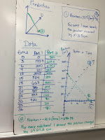
Our group's scenario this time was to release a buggy (traveling with constant velocity) at the same time as we released a ball on a ramp, so that the buggy would catch the ball at the bottom of the ramp. To make sure we didn't just time the ball and then time the car, Bryan told us he would decide how high up the ramp we'd be releasing the ball and would tell us right before it was time to start. We had to be ready to make a quick calculation of where the buggy had to start from in order to catch the ball. 

Once again, we divided into two groups: one to find the velocity of the car and one to find the acceleration of the ball on the ramp. Finding the velocity of the car was straight forward; we've done that plenty of times. But I was surprised to see the other half of our group timing to see how long it would take the ball to travel the full length of the ramp. That's how I'd find the average velocity, but that isn't useful at all. What they were doing, though, was quite smart. They were using a displacement equation we'd developed earlier which involved acceleration, and they were planning to plug in the displacement and the time to solve for it.

Once we had the acceleration of the ball and the velocity of the car, it was quite easy to write an equation for each. We even took the time to solve them for the variables we needed (time from the ball's equation and position from the car's equation).

Here's how we did:

So close! It hit the back of the car. If only we'd started the buggy 1 cm farther away...

Modeling Instruction in Physics: I had no idea...

You know, when I started this workshop, I thought I had a good idea of what Modeling Instruction was. After all, I'd read teacher blogs, looked at the AMTA website, checked out suggested course info that had been posted online, and been to a couple of workshops on it.

What I thought I knew about Modeling was entirely superficial and nowhere near as powerful. You know - students do the labs first, develop the formulas from their data, and then are better prepared for problem solving. Instead of me working hard to make examples and demos and clear explanations to get them to understand, they'd be doing the work by experiencing the phenomena themselves and thinking about it. Oh, and it's fun, so they like it!

Oh, there's so much more to it! There's a focus on drawing out student preconceptions and creating discrepant events to get them to analyze their own ideas. There's repeated exposure to the same ideas but in different contexts. There's unobtrusively guiding discussions so that 1) there isn't an authority figure and 2) they fully discuss their reasoning and (eventually) determine if it is faulty or not. 

I'm so glad I'm in this workshop!

I'm so nervous for this next school year!

Modeling Instruction in Physics: End of Week 1

This week has been one of the most intellectually stimulating weeks of my career. I've had so many thoughts going through my brain this week about the teaching I've done and the teaching I want to be doing.

First, it's well known that students come into class with preconceptions, based on their observations of the world, that don't match Newtonian physics. This was a theme in both my preparatory work and my graduate work. So I have some questions built into the beginning of some of my units to get an idea of what misconceptions my students have. But not all of my units. And I don't really use the questions I do have all that well. I try to remember to point out when something we just learned is contradictory to answers they gave on those preconception questions, and that's about it.

Those preconceptions students have are tenacious. Just pointing out and talking about them doesn't do much of anything. Students might modify those ideas slightly, but even that is unlikely. My students learn what to say on the tests and how to do the calculations they need to, but none that shows that they've changed their minds about how the world works. What I need are better questions and problems to introduce the contradictions between their thinking and what we observe, and my students to recognize that those contradictions exist and then work to find what the correct idea is.

Enter everything we've done this week. All of the labs and discussions are designed to bring different students' ideas out into the open and compare them with the physical data from the lab. Not just once, but over and over again.

Students will struggle with this. They will have trouble understanding each other's points and interpreting the data and graphs, and they will be confused. But nothing worthwhile is easy, and only ideas that more worthwhile and meaningful will replace what students already think. And what's more meaningful than an idea you came up with?

I love physics. I love watching the world around me and knowing why it works like it does. There's something awe-inspiring about how it all fits together. And I want my students to have that understanding. But I'm learning it has to be their work that gets them to that point, not mine. I can't take what I've learned from my efforts and distill it into simple phrases to tell them, and expect it to have any meaning for them. Instead, physics becomes nothing but empty phrases to parrot back and story problems to solve. There's no joy in that.

Modeling Instruction in Physics: Buggy Practicum

I had the most fun of the week on Day 3, during the Buggy Practicum.

We had to create one of three car crash action sequences for a "movie", and tell our director where to put the camera to film it. (The Academy Award goes to Bryan for his role as the penny-pinching director.) The group I was assigned to had to create a car chase that results in a rear-end crash in front of the camera. (Scenario 2) 

Adding to the excitement was the short amount of time we had to figure out where to put the camera. 

We didn't have much argument about how to start our work. Everyone jumped right in, setting up a 2 meter distance for the cars to travel and pulling out phones to be stopwatches. There were 4 or 5 of us timing, so we took the average time to use in each calculation of the cars' speeds. We used those speeds to set up motion equations based on the generalized equation we'd come up with earlier. 

This is where our group split into two. Some of us graphed the equations to see where they intersected. Others did some math to find the solution for the simultaneous linear equations. Then we checked that our answers matched.

It's funny. You know these two methods will both work, but it's still really exciting to find out other people reached the same answer you did, but in a completely different way. It's confidence inspiring. As a math teacher, I always say that answers are strongest when there are many ways to reach them. But as a physics teacher, I haven't been focusing on the multiple representations (graphs, equations, verbal explanations) as ways to reach a numerical answer. The verbal and graphical representations are for conceptual (qualitative) questions, while the math is how you reach an actual numerical answer. My students have been missing out on that moment of "Yeah, I got that too, but I used the graph." (They do compare numerical answers with each other... but it's just not the same as using a completely different method. They're mostly checking that they can do algebra correctly.)

Anyway, the best part of the practicum was actually testing our solution. Everyone gathered around to watch, and we all rooted for the crash to happen in the right spot, cheering when they crashed. From my vantage point, that crash definitely happened where it was supposed to. 

Unfortunately, our "director's"  camera disagreed. So close!!

I can appreciate the point Bryan made about failure. It is important to fail sometimes, and have to deal with that failure. Our cars didn't crash on the point we'd marked. We failed. 

But... I do wish we'd had time to explore what went wrong. There is instantaneous feedback built into the practicum (did it, or did it not, work), but a failure doesn't mean I don't understand the concepts involved. I'm pretty sure our work was right, and that it was a problem with releasing the cars simultaneously. Releasing the chase car early would account for an early crash. So, as an instructor, I think I'd want to make sure I had time built in to have a conversation with the groups about where their errors happened. And maybe let them try it again to see if they're right about those errors. (Not, of course, to change their "grade" on the practicum.)